Monetary policy and housing markets: insights using a novel measure of housing supply elasticity

This special feature explores how the responsiveness of new housing supply to house prices (the supply elasticity) affects the transmission of monetary policy. We document a long-term decline in the supply elasticity of new housing and find that a less elastic supply amplifies the impact of monetary policy on house prices compared with rents. This disparity could raise questions about the measurement of housing costs in inflation measures targeted by central banks, as typically rents, rather than house prices, directly enter consumer price indices. Our findings highlight the importance of considering changing housing supply conditions in monetary policy formulation¹.

JEL classification: E52, R31

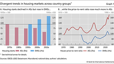
There have been strong secular trends in housing supply over the past few decades. In advanced economies (AEs), housing starts have been on a steady downward trend since the 1970s (Graph 1.A), accompanied by a rise in house prices relative to rents (Graph 1.B). This contrasts with the general trend in emerging market economies (EMEs) where housing starts have steadily ramped up since the 1990s, while the ratio of house prices to rents has remained more stable. These differences in housing supply conditions appear to play a crucial role in shaping the relationship between house prices and rents.

Against this backdrop, we explore how the responsiveness of new housing supply to price changes (the supply elasticity) influences the transmission of monetary policy to housing markets. As a first step, we develop time-varying measures of the supply elasticity for 21 economies, with data dating back to the 1970s in some cases. We approximate the supply of new housing with construction permits. We then analyse how the supply elasticity affects the transmission of monetary policy to house prices and rents. By incorporating time-varying elasticities, our analysis complements existing studies, which have relied on largely unchanging factors, such as geographical or regulatory constraints, to capture the elasticity. And by considering cross-country differences, our analysis extends existing studies, which focus on experience in the United States or only on house prices.²

Our results show that the supply elasticity influences the transmission of monetary policy to housing markets. When supply is less elastic, monetary policy easing has a larger impact on the price-to-rent ratio. This difference is almost entirely accounted for by the larger impact on house prices. Rents, by contrast, are much more sticky, irrespective of supply elasticity.

What could explain the findings? As in any other market, when supply is inelastic, more of the market adjustment to a change in demand – here monetary policy-induced – takes place through prices. This, in turn, could amplify the house price movements to the extent that it encourages households to extrapolate current house price growth into the future.

These findings have implications for policy. Where housing supply has become less elastic, the larger impact of monetary policy on house prices may strengthen the transmission through homeowners. As shown by Cloyne et al (2020), house price swings amplify especially the consumption response of mortgagors. Another implication arises from the larger disparity between the monetary impact on house prices and rents when housing supply is inelastic. As rents, rather than house prices, enter consumer price indices (CPIs) directly, this could raise questions about the measurement of housing costs in inflation measures targeted by central banks.³

This special feature proceeds as follows. The first section discusses our newly proposed measurement of housing supply elasticity. The second section analyses how the supply elasticity influences the transmission of monetary policy to housing markets and discusses potential mechanisms. The final section draws some policy implications.

Measuring housing supply elasticity

We estimate housing supply elasticity and how it changes over time using novel methods. Supply elasticity is a measure of how responsive housing supply is to changes in house prices. As it is not directly observable, it needs to be estimated. We estimate it using novel econometric techniques applied to data on house prices, building permits (as a proxy for new housing supply) and GDP (see Box A for details). The key idea behind our methodology is to identify demand shocks that push prices and quantities in the same direction, which allows us to trace the slope of the supply curve. Housing supply elasticity is then calculated as the ratio of the percentage change in building permits to the percentage change in house prices over the first quarter following a demand shock.⁴

Our elasticity estimates specifically measure the supply elasticity of new housing stock. As building permits capture the flow of the housing stock, our supply elasticity estimates implicitly assume that the marginal new addition to the housing stock determines the price of housing.⁵ The reliance on flow measures to compute supply elasticities is common in the literature. For example, Mayer and Somerville (2000b) use housing starts, while Caldera and Johansson (2013) use residential investment.

An advantage of our methodology is that it can trace the evolution of the supply elasticity over time. This is important because, as we show below, supply elasticities have changed significantly. By contrast, most of the literature has relied on measures that are time-invariant, for example based on geographical constraints (Saiz (2010)) or on regulatory and institutional constraints on land use (Glaeser et al (2005) and Gyourko et al (2008)).⁶

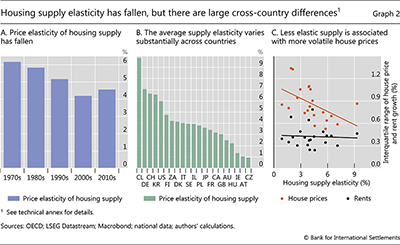
Our estimates indicate that the supply elasticity has declined over the past five decades on average (Graph 2.A). In the 1970s, a 1% increase in house prices would lead to an average increase in building permits of roughly 6%. By the 2000s, the average elasticity across countries had declined to close to 4%. It recovered slightly in the 2010s but remains well below its level in the 1970s. The decline in the elasticity has been attributed to a tightening in residential land use regulation (Gyourko et al (2021)) and to a drop in the productivity of the construction sector (Goolsbee and Syverson (2023)). Both factors can result in new housing becoming more costly and time-consuming to produce.⁷

Our results further indicate that the supply elasticity varies significantly across countries (Graph 2.B). Consistent with previous studies, the average supply elasticity is higher in the United States than in the United Kingdom.⁸ Although geographical constraints are often used to capture exogenous differences in supply elasticities (eg Saiz (2010)), the contrast between Switzerland and Austria, two mountainous countries, suggests that geography may not always be a useful proxy. Finally, there are large differences within AEs and EMEs. Among AEs, elasticities are high in Germany and the United States and low in Australia and Ireland. Among EMEs, they are high in Chile and South Korea and low in emerging Europe.⁹

Cross-country differences in house price dynamics provide a useful crosscheck on the validity of our supply elasticity estimates. A priori, one would expect that the more elastic the housing supply, the smaller the change in house prices for a given change in demand. Consistent with this logic, we find that house prices tend to be less volatile in countries with more elastic supply (Graph 2.C, downward sloping orange line). The flat black line, however, shows that the cross-country relationship does not extend to rents, hinting that the dynamics of rents in response to demand shocks, and hence also to monetary policy, might be quite different from that of house prices.

Monetary policy transmission to house prices and rents

The influence of housing supply: evidence from a panel of countries

To estimate how the supply elasticity affects the transmission of monetary policy to house prices and rents, we adapt the local projections (LP) methodology of Jordà (2005) to a panel of countries. Our sample includes 21 AEs and EMEs, covering the period between 1980 and 2019. Specifically, we estimate the following regressions for country c at month t up to horizon h = 0,...,24:

where y_c,t+h-y_c,t-1 is either the cumulative change in the logarithm of the house-price-to-rent ratio, the cumulative percentage change in house prices or the cumulative percentage change in rents; a_c^h is a country fixed effect which controls for time-invariant country characteristics such as land availability. X_c,t-1 is a set of country-specific controls dated t – 1 and earlier which includes changes in the dependent variable, GDP growth, the change in the policy rate, CPI inflation excluding housing, population growth and population density. When estimating the effect of monetary policy on house prices, we also include past changes in rents in the control set. Similarly for the effect on rents, we include past changes in house prices in the control set.¹⁰

To capture the impact of monetary policy on house prices and rents, we isolate changes in policy rates that are not correlated with the state of the economy. Specifically, we use monetary policy surprises, MP_c,t, from Choi et al (2024). These measures of interest rate surprises ensure that our estimates capture the impact of monetary policy itself, rather than the influence of other factors such as the state of the economy. The objects of interest are the coefficients β₁^h, which vary across low and high groups for the price elasticity of housing supply. Specifically, we construct variable I_c,t, which is a vector of indicator variables that sort the countries in our panel regression based on whether the country-specific mean elasticity in each decade is above or below the median in the cross section. The regression coefficients are plotted as impulse response functions with confidence bands based on standard errors clustered by country.

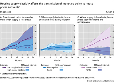
We find that the monetary policy impact on the house-price-to-rent ratio depends on the supply elasticity. Our estimates suggest that when supply is less elastic, the price-to-rent ratio increases by approximately 5% two years after a surprise 100 basis point fall in interest rates (Graph 3.A). When supply is elastic, the same monetary policy easing has a weaker effect, raising the price-to-rent ratio by around 2% in the first year, with the effect becoming statistically insignificant thereafter.¹¹

This difference in the impact of monetary policy is almost entirely accounted for by its larger impact on house prices. In countries where the housing supply is elastic, a 100 basis point reduction in policy rates results in only a modest 1.5% increase in house prices, which becomes statistically insignificant within a year (Graph 3.B). By contrast, when housing supply is less elastic, the increase in house prices is much stronger and long-lasting, with house prices increasing by around 5% two years after the rate cut (Graph 3.C).¹² We also found that a tightening of monetary policy does not exhibit any clear asymmetry compared with a loosening in low vs high supply elasticity countries. House prices react by more when supply is inelastic both when interest rates rise and when they fall.

Monetary policy has a much weaker impact on rents, regardless of the elasticity. Where supply is elastic, point estimates indicate that rents rise by a similar amount to house prices in response to a cut in interest rates, while they decline slightly when supply is inelastic. But in both cases the estimates are largely statistically insignificant.

The influence of housing supply: potential channels

If rents are sticky, monetary easing can push up house prices relative to rents. Under standard asset pricing logic, the price of a house equals the present discounted value of future rents. If rents do not respond much to monetary easing, a lower discount rate will push up house prices, raising the price-to-rent ratio.

If supply is inelastic, the overall house price increase following a monetary easing tends to be higher. This is because more of the housing market adjustment to lower interest rates is met by rising house prices rather than by adding new housing units. The fact that house prices adjust by more could additionally result in households extrapolating current house price growth into the future.¹³ Strong expectations of future house price growth tend to push up current house prices, which appears consistent with the sustained rise in house prices that we find in the data.

These mechanisms would rationalise the larger rise in house prices, but they struggle to explain why the response of rents is so limited. Assuming substitutability between owning and renting, one would also expect to see higher house prices translating into stronger rent increases when supply is inelastic. This, however, is not what we find in Graph 3. Of course, it is still possible that the adjustment in rents will occur over a much longer horizon than that in house prices.¹⁴ In addition, other forces such as landlords transforming rental units into owner-occupied ones could eventually bring rents more in line with house prices in the long run.

Policy considerations

Our findings have implications for monetary policy in countries with an inelastic housing supply. One implication is that in these countries, the greater impact of monetary policy on house prices may strengthen its transmission through homeowners. The larger changes in house prices can generate especially sizeable changes in the net worth of mortgagors who typically hold significant illiquid assets but have limited liquid wealth. As shown by Cloyne et al (2020), this amplifies their consumption response to monetary policy easing.

That said, when supply is inelastic the strong impact on house prices, but limited traction on rents, could raise questions about the measurement of housing costs in inflation measures targeted by central banks. The public would see large rises in house prices following monetary easing, but at the same time, the component capturing housing costs in CPI would barely move. This is because rents are a major component of CPI, while house prices are typically not included (see Annex A). Communication challenges may be greater in countries that use the rental equivalence approach to impute owner-occupied housing costs in CPI, which effectively places a much larger weight on rents.

More generally, when there is limited monetary policy traction on rents, more of the adjustment burden of bringing inflation to target will fall on other components of CPI. Over the past two years, strong growth in the rental component of CPI has kept inflation high relative to inflation targets in many countries (Banerjee et al (2024)). Policymakers have been confronted by a choice between imposing a fast and costly adjustment on non-housing sectors or tolerating a slower and more gradual return of inflation to target.

Our analysis also highlights the role of broader policies that go beyond the toolkit of central banks. In countries with low or declining supply elasticities, there is scope for supply-side interventions, such as regulatory reforms, that would boost the responsiveness of housing supply to positive aggregate demand shocks. Policy measures that aim to increase the productivity of the construction industry could also help ensure better alignment between supply and demand. Such policies could substantially alleviate the challenges for central banks generated by declining housing supply elasticities.

References

Aastveit, K, B Albuquerque and A Anundsen (2023): "Changing supply elasticities and regional housing booms", Journal of Money, Credit and Banking, vol 55, no 7, pp 1749–83.

Aastveit, K and A Anundsen (2022): "Asymmetric effects of monetary policy in regional housing markets", American Economic Journal: Macroeconomics, vol 14, no 2, pp 499–529.

Adam, K, O Pfäuti and T Reinelt (2024): "Subjective house price expectations, falling natural rates, and the optimal inflation target", Journal of Monetary Economics, August, 103647.

Albuquerque, B, M Iseringhausen and F Opitz (2024): "The housing supply channel of monetary policy", ESM Working Papers, no 59, February.

Andaloussi, M, N Biljanovska, A De Stefani and R Mano (2024): "Feeling the pinch? Tracing the effects of monetary policy through housing markets", IMF World Economic Outlook, chapter 2, April, pp 43–63.

Banerjee, R, D Gorea, D Igan and G Pinter (2024): "Housing costs: a final hurdle in the last mile of disinflation?", BIS Bulletin, no 89, July.

Baumeister, C and G Peersman (2013): "The role of time-varying price elasticities in accounting for volatility changes in the crude oil market", Journal of Applied Econometrics, vol 28, no 7, pp 1087–109.

Bureau of Labour Statistics (BLS) (2024): "Measuring price change in the CPI: rent and rental equivalence", US Bureau of Labour Statistics Factsheet.

Caldera, A and Å Johansson (2013): "The price responsiveness of housing supply in OECD countries", Journal of Housing Economics, vol 22, no 3, pp 231–49.

Central Statistics Office (CSO) (2014): Report of the Group of Technical Advisory Committee on Statistics of Prices and Cost of Living, Central Statistics Office, India.

Choi, S, T Willems and S Y Yoo (2024): "Revisiting the monetary transmission mechanism through an industry-level differential approach", Journal of Monetary Economics, vol 145, July, 103556.

Cloyne, J, C Ferreira and P Surico (2020): "Monetary policy when households have debt: new evidence on the transmission mechanism", Review of Economic Studies, vol 87, no 1, pp 102–29.

Dias, D and J Duarte (2019): "Monetary policy, housing rents and inflation dynamics", Journal of Applied Econometrics, vol 34, no 5, pp 673–87.

Duca, J, J Muellbauer and A Murphy (2021): "What drives house price cycles? International experience and policy issues",  Journal of Economic Literature, vol 5, no 3, pp 773–864.

Eiglsperger, M, I Ganoulis, B Goldhammer, O Kouvavas, M Roma and A Vlad (2024): "Owner-occupied housing and inflation measurement", ECB Statistics Paper Series, no 47, June.

Foote, C, L Loewenstein and P Willen (2021): "Cross-sectional patterns of mortgage debt during housing boom: evidence and implications", Review of Economic Studies, vol 88, no 1, pp 229–59.

Glaeser, E, J Gyourko and R Saks (2005): "Why is Manhattan so expensive? Regulation and the rise in housing prices", Journal of Law and Economics, vol 48, no 2, pp 331–69.

Goolsbee, A and C Syverson (2023): "The strange and awful path of productivity in the US construction sector", NBER Working Papers, no 30845, January.

Gorea, D, B Hofmann, D Igan and J Lee (forthcoming): "Housing supply elasticities across time and space and media sentiment towards new supply", mimeo.

Green, R, S Malpezzi and S Mayo (2005): "Metropolitan-specific estimates of the price elasticity of supply of housing, and their sources", American Economic Review, vol 95, no 2, pp 334–39.

Gyourko, J, J Hartley and J Krimmel (2021): "The local residential land use regulatory environment across US housing markets: evidence from a new Wharton index", Journal of Urban Economics, vol 124, July, 103337.

Gyourko, J, A Saiz and A Summers (2008): "A new measure of the local regulatory environment for housing markets: the Wharton Residential Land Use Regulatory Index", Urban studies, vol 45, no 3, pp 693–729.

Irving Fischer Committee on Central Bank Statistics (IFC) (2006): "Proceedings of the IFC Workshop on 'CPI measures: central bank views and concerns", IFC Bulletin, no 24, August.

Jordà, Ò (2005): "Estimation and inference of impulse responses by local projections", American Economic Review, vol 95, no 1, pp 161–82.

Loewenstein, L and P Willen (2023): "House prices and rents in the 21st century", NBER Working Papers, no 31013, March.

Malpezzi, S and D Maclennan (2001): "The long-run price elasticity of supply of new residential construction in the United States and the United Kingdom", Journal of Housing Economics, vol 10, no 3, pp 278–306.

Mayer, C and C T Somerville (2000a): "Land use regulation and new construction", Regional Science and Urban Economics, vol 30, no 6, pp 639–62.

Mayer, C and C T Somerville (2000b): "Residential construction: using the urban growth model to estimate housing supply", Journal of Urban Economics, vol 48, no 1, pp 85–109.

Saiz, A (2010): "The geographic determinants of housing supply", Quarterly Journal of Economics, vol 125, no 3, pp 1253–96.

Sommer, K, P Sullivan and R Verbrugge (2013): "The equilibrium effect of fundamentals on house prices and rents", Journal of Monetary Economics, vol 60, no 7, pp 854–70.

Annex A: Rents and measurement of housing costs in CPIs

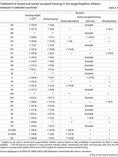
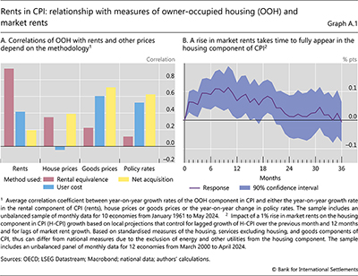
Housing costs are a major part of consumer price indices (CPIs), so the effect of monetary policy on housing markets extends beyond indirect effects on household demand. The overall housing cost component constitutes around 21% of CPI baskets on average (Table A.1). Even after subtracting costs for energy and other utilities, housing cost for rents and owner-occupied housing (OOH) still often make up around 14% of CPI baskets on average.¹⁵

Rents are the single most important underlying variable feeding into CPI housing costs. Direct expenditures on rents actually paid by households make up around 7% of CPI baskets on average. In addition, rents are often the key variable determining the costs of OOH when it is included in the CPI. In particular, the rental equivalence method is by far the most common way in which statistical agencies include OOH in CPI baskets, with an average weight of around 14% (Table A.1, third column). The rental equivalence method answers the hypothetical question, "How much rent would I demand if I were to rent my home instead of live in it?". To compute the answer to this question, statistical agencies use data on actual rents paid on equivalent housing in the rental sector. Unsurprisingly, there is an almost perfect correlation between actual rents paid and OOH costs as captured by the rental equivalence approach (Graph A.1.A).

In this special feature, we use rent estimates that statistical agencies used to calculate CPI, but there are important measurement issues to consider. CPI rents capture actual rents paid by all households in rental accommodation, which includes ongoing tenancies as well as newly let properties. The CPI rent data, however, have a drawback because sampling methodologies can lead to artificially smooth rents data over short horizons, as it takes time for statistical agencies to capture all changes in rents.¹⁶ To assess the extent of this "fake" persistence in rents, we assess the dynamic relationship between rents on newly let properties and CPI rents for a limited set of countries where we have both series (Graph A.1.B). The co-movement between rents on newly let properties and CPI rents peaks at around six months, suggesting that the CPI rent data will capture the cumulative effect of any rent changes only after about six months. Thus, in our analysis of the impact of monetary policy it is important to look at the impact on rents at horizons longer than six months to assess the overall effects.

While house prices themselves do not directly enter CPI measures of housing costs, they are relatively well correlated with some measures of OOH (Graph A.1.A). The net acquisition approach is the most strongly correlated with house prices. It captures the cost of living in an owner-occupied home by the price of newly built housing excluding the value of the land upon which the house stands. Both the net acquisition and user cost measures of OOH costs are also strongly correlated with goods price inflation and interest rates, unlike the rental equivalence approach.

Technical annex

Graph 1.A: GDP-PPP-weighted average across 11 advanced economies (AEs) and six emerging market economies (EMEs).

Graph 1.B: GDP-PPP-weighted average across 14 AEs and seven EMEs. The house-price-to-rent ratio is computed for each economy based on house price indices that use prices for both new and existing dwellings and rent indices constructed using CPI data.

Graph 2.A: GDP-PPP-weighted average across 21 countries (shown in Graph 2.B), computed using a smaller set of countries when data are not available.

Graph 2.B: The average is computed based on varying time periods for each country, depending on data availability. As a consequence, countries for which the data start later in the sample period 1970–2019 (eg Austria and Czechia) tend to have lower elasticities, in line with the evidence shown in Graph 2.A.

Graph 2.C: The sample includes the countries shown in Graph 2.B. For any given country, each dot shows the average estimated supply elasticity and the interquartile range of monthly growth of house prices or rents, deflated by CPI excluding housing. The orange fitted line indicating the relationship between supply elasticity and house price volatility is significant at the 5% level.

Graph 3: Estimates are derived from local projections that regress the cumulative percentage change in the logarithm of the house-price-to-rent ratio, house prices or rents on monetary policy surprises of 100 basis points. The sample includes an unbalanced panel of 21 economies from 1980 to 2019. Economies are categorised as having low (high) supply elasticity if the decadal elasticity of housing supply is lower (higher) than the cross-sectional median.

¹  The views expressed are not necessarily those of the Bank for International Settlements. We thank Burcu Erik for excellent research assistance. For helpful comments, we are also grateful to Frederic Boissay, Claudio Borio, Mathias Drehmann, Gaston Gelos, Boris Hofmann, Enisse Kharroubi, Emanuel Kohlscheen, Benoît Mojon, Daniel Rees, Tom Rosewall, Andreas Schrimpf and Hyun Song Shin. All remaining errors are ours.

²   For example, Dias and Duarte (2019) study the effect of monetary policy shocks on rents in the United States, while Aastveit and Anundsen (2022) and Albuquerque et al (2024) assess how geographical and regulatory differences across US states influence the monetary transmission to house prices and rents, respectively. Andaloussi et al (2024) examine how cross-country differences in population density influences the transmission of monetary policy to house prices.

³   See Annex A, which highlights the importance of rents in CPI baskets. In many economies, rents are also used to measure the costs of owner-occupied housing.

⁴   We also experimented with elasticity measures based on the cumulative responses over four quarters following a demand shock. We found that the properties of these elasticities do not differ much from those based on the contemporaneous responses.

⁵   The flow of new housing can even capture changes in the per capita housing stock, for example due to population growth or the need to replenish depreciated housing units (Foote et al (2021) and Loewenstein and Willen (2023)).

⁶   A separate strand of the literature estimates the supply elasticity by regressing changes in the housing stock on changes in prices (Mayer and Somerville (2000a) and Green et al (2005)). However, there are endogeneity issues with this older approach because it also captures how exogenous changes in housing supply affect future prices.

⁷   Aastveit et al (2023) estimate measures of supply elasticity using an instrumental variables regression for 254 US metropolitan statistical areas spanning the housing boom episodes of 1996–2006 and 2012–19. They also find that the elasticity has been declining over time.

⁸   See eg Malpezzi and Maclennan (2001).

⁹   Our elasticity estimates for some countries differ from those in Caldera and Johansson (2013) due to differences in sample periods and in how new housing supply is measured, ie building permits vs residential investment. See Duca et al (2021) for a more detailed discussion of approaches used in the literature to calculate the supply elasticity and the reasons behind differences in elasticity estimates.

¹⁰  We do not control for past changes in house prices or rents when estimating the effects on the price-to-rent ratio, as prices and rents are highly correlated with past changes in the dependent variable, which is included as a control in X_c,t-l.

¹¹  Our results are robust to a variety of different specifications, including grouping countries based on their elasticities in a given quarter, rather than over the decade; using growth in housing starts as an alternative measure of housing supply instead of our baseline supply elasticity estimates; and using supply elasticities from housing-specific demand shocks to rank countries into low and high groups.

¹²  The response peaks at close to 6% three and half years after the monetary policy shock.

¹³  See Adam et al (2024), who find that house price expectations become more extrapolative when the price-to-rent ratio is high.

¹⁴  Another channel could run through credit constraints if they are more binding when supply is less elastic (Albuquerque et al (2024)). Sommer et al (2013) present a model in which the supply and demand in rental markets are jointly determined alongside the demand for owner-occupied housing. When interest rates and down payment requirements fall (eg due to more ample credit supply), the demand for rental units by tenants falls because home ownership becomes cheaper. At the same time, the supply of rental property from landlords increases because investment in rental property becomes more attractive relative to saving in deposits.

¹⁵  Housing costs in the CPI often also include energy and other utility costs, which make up around 7% of the CPI basket on average.

¹⁶  To ensure comparability over time, statistical agencies sample rents from the same dwellings. To limit data collection costs and since rents change infrequently, they do not gather rent data for the same household every month. Instead, they divide the sample into subgroups and typically sample each subgroup every six months. See, for instance, BLS (2024) and CSO (2014) for descriptions of the rent sampling methodology in the United States and India, respectively. This means that if the rent of a dwelling increases one month after the sampling date, it will take statistical agencies another five months (the next sampling date) to incorporate this increase in the index.